EFP
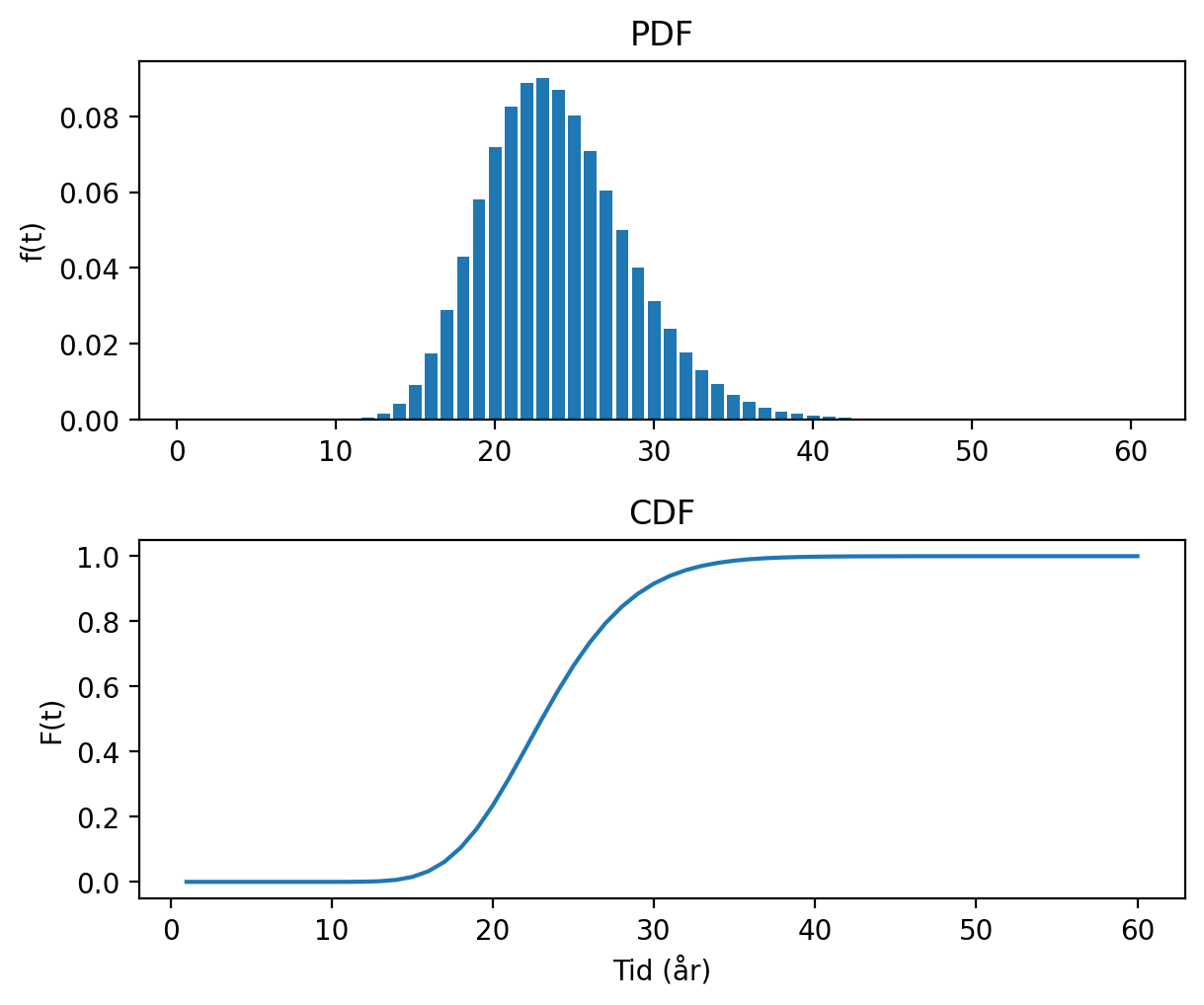
Denne metoden for å estimere sviktsannsynlighet bruker en levetidskurve som input, det vil si, estimater for gjennomsnittlig oppholdstid i hver tilstand (T) og tilhørende 10 persentiler (P10).
Denne notebooken er en oversatt versjon av EFP 1.3.3 fra Visual Basic med noen oppdateringer fra EFP 3.0 og 3.1.
Nyttige referanse:
Heggset, J. et al. (2009). User’s Guide to Optimal Maintenance Tool Box - Version 2
Welte, T. (2008). A rule‑based approach for establishing states in a Markov process applied to maintenance modelling. Proceedings of the Institution of Mechanical Engineers, Part O: Journal of Risk and Reliability, 223(1), 1–12
Rausand, M. (2021). System reliability theory: Models, statistical methods, and applications (3rd ed.). Wiley.
Source
import numpy as np
from scipy.stats import gamma
import matplotlib.pyplot as plt
from scipy.optimize import root_scalar
from scipy.linalg import expm
%config InlineBackend.figure_format = 'retina'
Definer levetidskurve
labels = ['T1', 'T2', 'T3', 'T4']
Tbar = [30, 10, 10, 5]
P10 =  [25, 8, 6, 2]
Source
start = 0
positions = []
for t in Tbar:
    end = start + t
    positions.append((start, end))
    start = end
fig, ax = plt.subplots(figsize=(7, 3))
for i, (start, end) in enumerate(positions):
    ax.plot([start, end], [5-i, 5-i], lw=8)
    ax.text((start + end) / 2, 1.1, labels[i], ha='center', va='bottom', fontsize=12)
ax.plot(np.concatenate(([0],np.cumsum(Tbar[0:5]))),[5,4,3,2,1],'r-*')
ax.set_ylim(0, 6)
ax.set_xlim(0, positions[-1][1] + 5)
ax.set_yticks([5,4,3,2,1])
ax.set_yticklabels(['1','2','3','4',''])
ax.set_xticks(np.concatenate(([0],np.cumsum(Tbar[0:5]))))
ax.set_xlabel('Tid (år)')
ax.set_ylabel('Tilstand (TK)')
plt.title('Levetidskurve', fontsize=14)
plt.grid()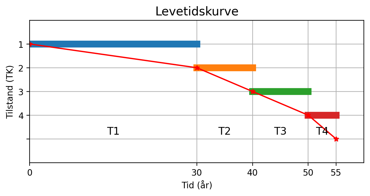
Source
def fit_gamma_from_mean_p10(mean_life, p10):
    mean_life = np.atleast_1d(mean_life).astype(float)
    p10 = np.atleast_1d(p10).astype(float)

    if len(mean_life) != len(p10):
        raise ValueError(
            "mean_life and p10 must have the same length"
        )

    alpha = np.zeros(len(mean_life))
    theta = np.zeros(len(mean_life))

    for i, (m, p) in enumerate(zip(mean_life, p10)):

        def objective(a):
            b = m / a
            return gamma.cdf(p, a, scale=b) - 0.10

        result = root_scalar(
            objective,
            bracket=[0.1, 100],
            method="brentq"
        )

        alpha[i] = result.root
        theta[i] = m / alpha[i]

    if len(alpha) == 1:
        return alpha[0], theta[0]

    return alpha, theta
Finn beste gammaparametre for alle ekspertvurderinger og plot
alpha,theta = fit_gamma_from_mean_p10(Tbar, P10)

print("alpha = ",np.round(alpha,2))
print("theta = ",np.round(theta,2))
alpha = [56.21 38.57 8.82 3.43]
theta = [0.53 0.26 1.13 1.46]
Source
x = np.linspace(0, 40, 200)
fig, axes = plt.subplots(1, figsize=(9, 3)) # 1 rad, 2 kolonner
for i in range(len(alpha)):
y = gamma.pdf(x, alpha[i], scale=theta[i])
axes.plot(x, y, label=f'{labels[i]} (alpha={alpha[i]:.2f}, theta={theta[i]:.2f})')
axes.legend()
axes.set_xlabel('Tid (år)')
axes.set_ylabel('f(t)')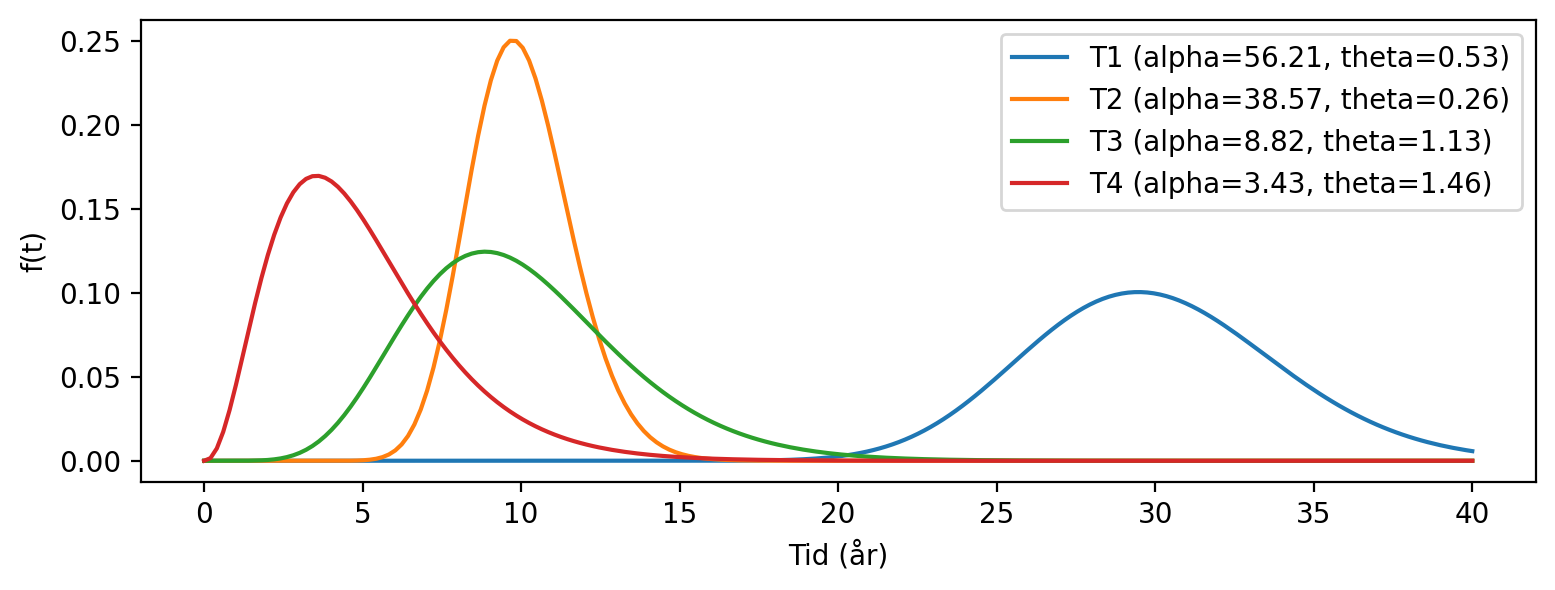
Source
def find_efirst_elast(alpha, theta, mean_times):
s_states = np.ceil(alpha).astype(int)
efirst = np.zeros(len(alpha))
elast = np.zeros(len(alpha))
for i in range(len(alpha)):
E = mean_times[i]
s = s_states[i]
var = alpha[i] * theta[i] ** 2
H = (E * (s - 1)) ** 2 - (s**2 - s) * (E**2 - var)
H = max(H, 0)
el = E - (s - 1) * (E * (s - 1) + np.sqrt(H)) / (s**2 - s)
ef = (E - el) / (s - 1)
efirst[i] = ef
elast[i] = el
return efirst, elast
def define_markov_chain(start_state, alpha, efirst, elast):
ss = np.ceil(alpha).astype(int)
if start_state == 'ny':
first_state = 1
first_sub = 1
else:
level = 1 if '+' in start_state else 2 if start_state[-1].isdigit() else 3
first_state = int(start_state[0])
first_sub = int(np.floor(((2 * level - 1) / 6) * ss[first_state - 1]) + 1)
durations = []
for state in range(first_state, 5):
end_sub = ss[state - 1]
for sub in range(first_sub, end_sub + 1):
durations.append(
elast[state - 1] if sub == end_sub else efirst[state - 1]
)
first_sub = 1
durations.append(0.0)
durations = np.asarray(durations)
lam = np.zeros_like(durations)
mask = durations > 0
lam[mask] = 1.0 / durations[mask]
return durations, lam
def calculate_mttf(durations):
return np.sum(durations[:-1])
def BuildGeneratorMatrix(lam):
"""
Continuous-Time Markov Chain generator matrix.
Last state is absorbing (failure state).
"""
n = len(lam)
Q = np.zeros((n, n))
for i in range(n - 1):
Q[i, i] = -lam[i]
Q[i, i + 1] = lam[i]
return Q
def CalculateProbCTMC(Q, Tmax=60):
"""
Exact CTMC solution using matrix exponential.
"""
n = Q.shape[0]
p0 = np.zeros(n)
p0[0] = 1.0
cdf = np.zeros(Tmax)
pdf = np.zeros(Tmax)
prev_fail = 0
for t in range(1, Tmax + 1):
Pt = expm(Q * t)
p = p0 @ Pt
fail_prob = p[-1]
cdf[t-1] = fail_prob
pdf[t-1] = fail_prob - prev_fail
prev_fail = fail_prob
return cdf, pdf
def CalculateProbAlder(age, lam, Tmax=60):
#
# Build CTMC generator matrix
#
Q = BuildGeneratorMatrix(lam)
n = Q.shape[0]
#
# Initial state (new asset)
#
p0 = np.zeros(n)
p0[0] = 1.0
#
# Distribution at current age
#
p_age = p0 @ expm(Q * age)
#
# Condition on survival to current age
#
R_age = 1.0 - p_age[-1]
if R_age <= 1e-12:
raise ValueError(
f"Survival probability at age {age} is approximately zero."
)
p_age[:-1] /= R_age
p_age[-1] = 0.0
#
# Future failure distribution
#
cdf = np.zeros(Tmax)
pdf = np.zeros(Tmax)
previous_failure = 0.0
for t in range(1, Tmax + 1):
#
# t years from today
#
p_future = p_age @ expm(Q * t)
failure_probability = p_future[-1]
cdf[t - 1] = failure_probability
pdf[t - 1] = failure_probability - previous_failure
previous_failure = failure_probability
return Tmax, cdf, pdfE1, E2 = find_efirst_elast(alpha, theta, Tbar)Source
positions = []
time_ticks = [0]
start = 0
ss = np.ceil(alpha).astype(int)
for i in range(4):
total_length = (ss[i]-1)*E1[i] + E2[i]
end = start + total_length
positions.append((start, end))
time_ticks.append(end)
start = end
fig, ax = plt.subplots(figsize=(8, 2))
colors = plt.rcParams['axes.prop_cycle'].by_key()['color']
for i, (start, end) in enumerate(positions):
color = colors[i % len(colors)]
n_parts = ss[i]
x = start
for j in range(n_parts):
width = E1[i] if j < n_parts - 1 else E2[i]
ax.add_patch(plt.Rectangle((x, 0.95), width, 0.1, color=color))
ax.plot([x, x], [0.9, 1.1], color='black', lw=0.8)
x += width
ax.plot([end, end], [0.9, 1.1], color='black', lw=0.8)
ax.text((start + end) / 2, 1.15, labels[i], ha='center', va='bottom', fontsize=12)
ax.set_ylim(0.85, 1.3)
ax.set_xlim(0, positions[-1][1] + 5)
ax.set_yticks([])
ax.set_xticks(np.round(time_ticks,0))
ax.set_xticklabels([str(t) for t in np.round(time_ticks,0)])
ax.tick_params(axis='x', length=5)
ax.set_xlabel('Tid (år)')
plt.title('Levetidskurve med deltilstander', fontsize=14)
plt.tight_layout()
plt.show()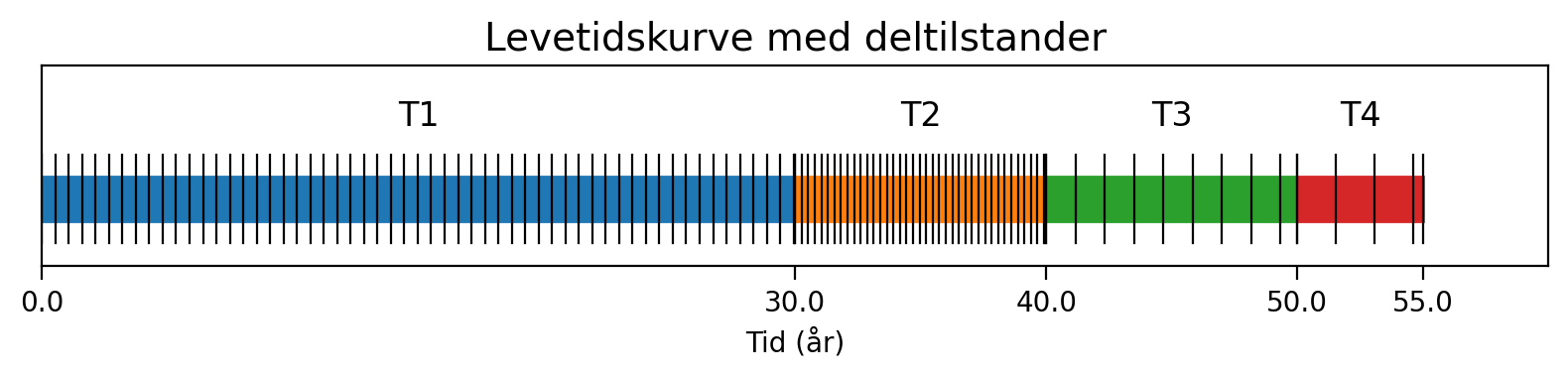
Angi nåværende tilstand eller alder
mode = 'state_mode'
start_state = "2+" # {'ny',1+,1,1-,2+,2,2-,3+,3,3-,4+,4,4-}
age = 19Source
durations, lam = define_markov_chain(
start_state,
alpha,
E1,
E2,
)
Q = BuildGeneratorMatrix(lam)
if mode == 'state_mode':
# state-based
cdf, pdf = CalculateProbCTMC(Q, Tmax=60)
mttf = calculate_mttf(durations)
else:
# age-based
simPeriod, cdf, pdf = CalculateProbAlder(
age,
lam,
Tmax=60
)
mttf = np.sum(1 - cdf)
#print("Age:", age)
print("Expected remaining life =", round(mttf, 1), "years")
print('alpha =', np.round(alpha, 2))
print('theta =', np.round(theta, 2))
t = np.arange(1, len(pdf) + 1)
fig, ax = plt.subplots(2, 1, figsize=(6, 5))
ax[0].bar(t, pdf)
ax[0].set_title('PDF')
ax[1].plot(t, cdf)
ax[1].set_title('CDF')
plt.tight_layout()
ax[1].set_xlabel('Tid (år)')
ax[1].set_ylabel('F(t)')
ax[0].set_ylabel('f(t)')
plt.show()
print('')Expected remaining life = 23.4 years
alpha =  [56.21 38.57  8.82  3.43]
theta =  [0.53 0.26 1.13 1.46]